
Advanced statistical tools and methods
We do research ourselves on several aspects of Advanced statistical tools and methods. Here I break down our research by the subject focus with short highlights of our findings.- Wavelet coherence
- Singular Spectrum Analysis
- Wavelet lag coherence
- Significance testing
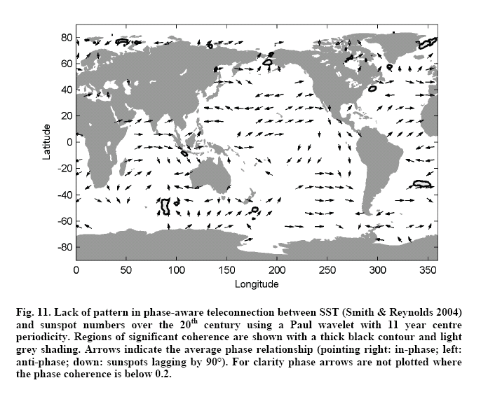
- Phase-aware teleconnections
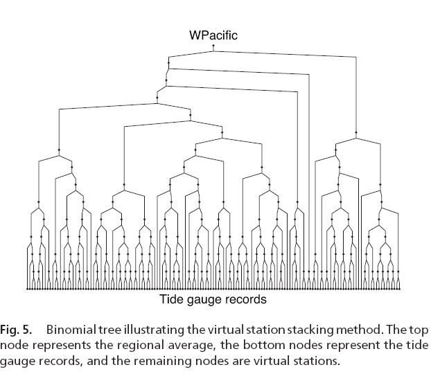
- Virtual station spatial stacking
- Normalization
- PCA significance
- Climate research
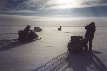
- Glaciology reserach
Zhihua Zhang in my group in GCESS, BNU, has produced several papers in 2011 and 2012 on wavelet significance testing, the influence of the COI, and works on different wavelets. This work is important in paleoclimate research since the significance of signals is easily mistaken.
New significance test methods for Fourier analysis of geophysical time series
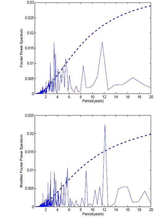
When one applies the discrete Fourier transform to analyze finite-length time series, discontinuities at the data boundaries will distort its Fourier power spectrum. In this paper, based on a rigid statistics framework, we present a new significance test method which can extract the intrinsic feature of a geophysical time series very well. We show the difference in significance level compared with traditional Fourier tests by analyzing the Arctic Oscillation (AO) and the Nino3.4 time series. In the AO, we find significant peaks at about 2.8, 4.3, and 5.7 yr periods and in Nino3.4 at about 12 yr period in tests against red noise. These peaks are not significant in traditional tests
The figure shows (Top) Fourier power spectrum of Nino3.4 indices is computed by discrete Fourier transform. (Bottom) Modified Fourier power spectrum of Nino3.4 indices is computed by our method. The dashed line is 95% confidence red noise spectrum
Empirical Mode Decomposition and Significance Tests of Temperature Time Series discusses Empirical mode decomposition (EMD) has become a powerful tool for adaptive analysis of non-stationary and nonlinear time series. In this paper, we perform a multi-scale analysis of the Central England Temperature and the proxy temperature from Greenland ice core time series by using EMD. We make a significance test against the null hypothesis of red noise and determine both the dominant modes of variability and how those modes vary in time
Distribution of Fourier power spectrum of climatic background noise, In 1998, Torrence and Compo [1] provided an empirical formula on the distribution of Fourier power spectrum of red noise which is the foundation of significance tests on Fourier analysis of climatic signals. In this paper, we prove this empirical formula in a rigorous statistical framework, and apply it to significance tests of central England temperatures
Intrinsic feature extraction in the COI of wavelet power spectra of climatic signals,
Since the wavelet power spectra are distorted at data boundaries (the cone of influence, COI), using traditional methods, one cannot judge whether there is a significant region in COI or not. In this paper, with the help of a first-order autoregressive (AR1) extension and using our simple and rigorous method, we can obtain realistic significant regions and intrinsic feature in the COI of wavelet power spectra. We verify our method using the 300 year record of ice extent in the Baltic Sea.
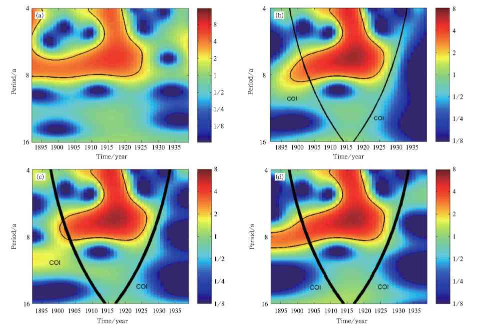 The figure shows wavelet power spectrum of Southern Greenland winter temperature indices is obtained by using: (a) full-length
data, (b) "zero-padding" method, (c) "even-padding" method, and (d) our method. The black contour designates the 90%
signi¡¥cance level against red noise, and COI is just the region below the thick line.
The figure shows wavelet power spectrum of Southern Greenland winter temperature indices is obtained by using: (a) full-length
data, (b) "zero-padding" method, (c) "even-padding" method, and (d) our method. The black contour designates the 90%
signi¡¥cance level against red noise, and COI is just the region below the thick line.Improved significance testing of wavelet power spectrum near data boundaries as applied to polar research, When one applies the wavelet transform to analyze finite-length time series, discontinuities at the data boundaries will distort its wavelet power spectrum in some regions which are defined as a wavelength-dependent cone of influence (COI). In the COI, signinifcance tests are unreliable. At the same time, as many time series are short and noisy, the COI is a serious limitation in wavelet analysis of time series. In this paper, we will give a method to reduce boundary effects and discover significant frequencies in the COI. After that, we will apply our method to analyze Greenland winter temperature and Baltic sea ice. The new method makes use of line removal and odd extension of the time series. This causes the derivative of the series to be continuous (unlike the case for other padding methods). This will give the most reasonable padding methodology if the time series being analyzed has red noise characteristics.
Aslak Grinsted's thesis contains much of our development of statistical tools
The wavelet coherence website contains worked examples of the use of this powerful tool for examining pairs of time series.
As this example shows with the relationship between Central England Temperatures (CET) and Southern Oscillation Index (SOI).
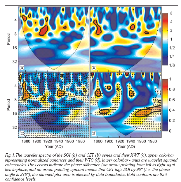
See Moore et al., 2005 for more discussion.
We have used the wavelet coherence method in about 9 papers :
Description of method: Grinsted et al. 2004;
Sea level links to AO and NAO: Jevrejeva et al. 2005
Methods and SSA trends: Moore et al., 2005
Global sea level reconstruction: Jevrejeva et al. 2006
(No) solar forcing of AO and ENSO: Moore et al. 2007
ENSO and AO impact on arctic sea ice: Jevrejeva et al. 2003
Transport of ENSO to polar regions: Jevrejeva et al. 2004
Solar forcing, QBO and AO: Moore et al. 2006a
SO4 and Ca links in ice core: Moore et al. 2006b.
Additionally
 we have made much use of Singular Spectrum Analysis
e.g. in processing ice radar data: Moore & Grinsted 2006
we have made much use of Singular Spectrum Analysis
e.g. in processing ice radar data: Moore & Grinsted 2006ENSO and AO impact on arctic sea ice: Jevrejeva et al. 2003
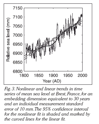
In particular we developed the method of estimating the confidence limits of the optimal non-linear trend of the data
Methods and SSA trends: Moore et al., 2005
Global sea level reconstruction: Jevrejeva et al. 2006
SSA trend analysis is a powerful tool with numerous advantages of traditional low pass filtering and polynomial or straight-line fitting as the confidence intervals are the smallest.
Wavelet lag coherence is a new method that we have developed that grew out of our work on Mean Phase Coherence (Moore et al. 2006a) to study possible causality by looking at the phase relationships between two time series. The idea being that if time series A really causes the variability in time series B then there should be a consistent phase relationship between them rather than simple correlation. Thus peaks and troughs in one time series A should always occur before corresponding features in B. This is best illustrated by an example:
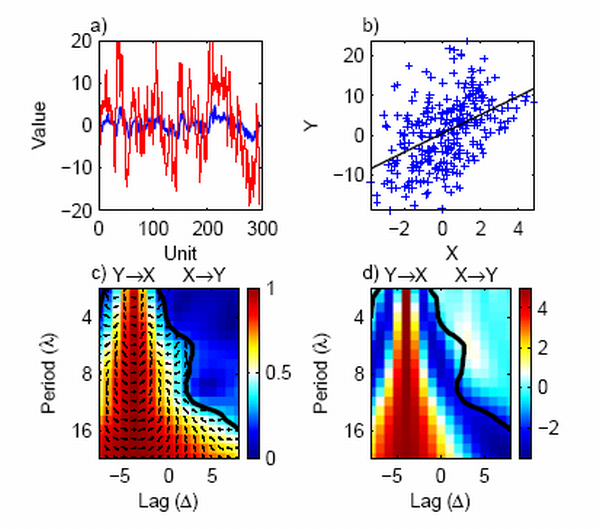
The example shows that for two signals that constructed such that X is red noise (that is each point is closely dependent on its immediate predecessor in time - which is reasonably true of most climate time series e.g. monthly air temperatures), with mean 0, unit variance and AR(1) of 0.8. Series Y is made from X multiplied by 5 and then X is lagged by 4 units relative to Y. So in a sense Y causes X.
The scatter plot of X and Y shows a totally misleading relationship between the two that fails to capture any real relationship between the two.
Plot C shows the mean phase coherence between the series - this is created using a wavelet decomposition of the timeseries, Monte-Carlo significance testing shows the 95% level as a thick contour, the arrow directions shows the relative phase angle so that the arrows pointing right at a lag of -4 (on the abscissa) means that the series are in phase at this lag. The label on the plot at negative lag indicates that Y leads X at that lag. The sensitivity in plot D shows that at a lag of -4, there is a factor of 5 between X and Y for all the different periods on the ordinate. Recently we have used the wavelet lag coherence method in two papers (in press) on Atlantic tropical cyclones
Significance testing
All studies referenced above employ significance testing. This is essential to produce answers that are meaningful. An answer with no uncertainty is worthless. Choice of appropriate significance test is not always obvious. It is very lamentable that most scientists have a very poor grasp of statistics - as we have often discovered during the review process for our paper. While sometimes it is possible to use theoretical assumptions about a particular data set e.g Normality, independence, autocorrelation etc., more often it is safer to use methods that rely on the observed data and estimate significance by Monte Carlo / Bootstrap / Jack-knife methods.
Some general points worth considering: For most time series data cannot be treated as though independent. Any data point value usually depends on the previous values. One of the simplest ways of accounting for such autocorrelation of data is to use a simple red noise background (see the example in wavelet lag coherence above). There are more complex autocorrelation models that use more than just the last immediate data point, but for every extra data used another parameter must be estimated, which in the typically short and noisy time series found in climate research means that the results often are no better determined for the increased complexity of the noise model - and may undermine the ability of the analysis to determine useful signal parameters.
Sometimes a fractal scaling noise background may be a better description of the data, however, this is a powerful way of removing any signal from a time series, as in a long enough series any finite step change in variables is somewhat likely to occur. So while this process is analytically simple to include as a noise background, careful thought should be given before using it.
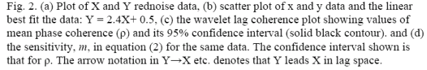
Perhaps the best illustration is from the volcanic impact on sea level paper where we develop in the supplementary information a bespoke method for jacknife on rednoise.
Another example often misunderstood is in ice core chemical analysis where often the analysis method used is ion chromatography. This method has errors that are proportional (to good approximation) to the measured value, so usually a percentage error is quoted (typically about 5%). However while the errors are not constant, there is way that a good standard deviation can be given for the set of measurements of concentrations along an ice core. In order to be able to process the data using statistical methods like regression analysis, the errors in the data must be made equal. This is easily done in this case by taking the logarithm of the concentration data. The errors will then be independent of the measured value and so can be used in regression analyses etc.
 This has also applicability to various methods such as the correction to remove
sea salt input to chemical species, which are usually taken as a simple fractions
based on e.g. sodium concentrations. This is incorrect, and the removal should
be done log space not concentration space. Another erroneous assumption is that
selecting spikes greater than 2 or 3 standard deviations selects data extremely
unlikely to occur by chance - but the assumption relies on concentration data
being Normal, whereas in fact the data are really Log normal.
This has also applicability to various methods such as the correction to remove
sea salt input to chemical species, which are usually taken as a simple fractions
based on e.g. sodium concentrations. This is incorrect, and the removal should
be done log space not concentration space. Another erroneous assumption is that
selecting spikes greater than 2 or 3 standard deviations selects data extremely
unlikely to occur by chance - but the assumption relies on concentration data
being Normal, whereas in fact the data are really Log normal. This is illustrated in the figure where the sulphate residuals found in log space are calculated by trying to regress sulphate against other ions in an ice cores. The large spikes are places where the model fit was very poor due the presence of a sudden large sulphate input in the ice - almost certainly a result of a volcanic eruption. Independent dating of the core showed that the dates of the sulphate spikes correspond closely (2% errors) to those of known very large volcanic eruptions - identified by the labels above the spikes - see Moore et al. 2006b for details.
Additionally we have been developing novel time series methods such as phase-aware teleconnections Jevrejeva et al. 2003; Grinsted, 2006; Moore et al. in press J. Climate);
These are made by mapping the phase coherence and the mean relative phase between two series
Virtual station spatial stacking is a method that optimally stacks time series from different stations located around the earth, such as tide gauge stations (Jevrejeva et al. 2006; Grinsted et al. 2006)
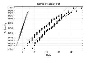
Normalization is a drastic but fail safe procedure to convert any pdf into a Normal distribution. A Matlab routine to do it can be downloaded here
 The transformation operator is optimally chosen so that the new probability
density function is Normal, has zero mean and unit variance. This is calculated
by making the inverse normal cumulative distribution function of the percentile
distribution of the original distribution. We refer to this procedure
as Normalization and it can be a rather drastic operation to use on a time series.
However, Jevrejeva et al. 2003
have shown that the results from
even grossly non-Normal distributions, that would not produce reliable results
with the wavelet method, do give results after Normalization that are consistent
with alternative methods of signal extraction such as Singular Spectrum Analysis.
The figure shows raw Atlantic Tropical Cyclone counts (TC) data (diamonds),
(from Mann et al., 2007) modified TC (squares), (from Landsea, 2007) and
Normalized modified TC (TC") (marked by +), plotted on normal probability
scaling so that straight lines represent a Normal probability distribution.
The transformation operator is optimally chosen so that the new probability
density function is Normal, has zero mean and unit variance. This is calculated
by making the inverse normal cumulative distribution function of the percentile
distribution of the original distribution. We refer to this procedure
as Normalization and it can be a rather drastic operation to use on a time series.
However, Jevrejeva et al. 2003
have shown that the results from
even grossly non-Normal distributions, that would not produce reliable results
with the wavelet method, do give results after Normalization that are consistent
with alternative methods of signal extraction such as Singular Spectrum Analysis.
The figure shows raw Atlantic Tropical Cyclone counts (TC) data (diamonds),
(from Mann et al., 2007) modified TC (squares), (from Landsea, 2007) and
Normalized modified TC (TC") (marked by +), plotted on normal probability
scaling so that straight lines represent a Normal probability distribution.
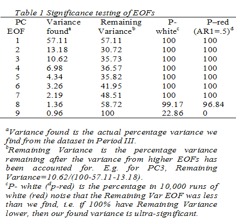
PCA significance One key element in Principle Component Analysis is to determine how significant each of the resolved components are, and hence where to define a noise floor, beyond which interpretation is meaningless. Moore and Grinsted, 2008 discuss two methods.
 One is based on the signal to noise ratio of the series,
the other method is to examine the median and 95% confidence intervals of the
Principle Components (PCs), (using the median rather than the mean makes for a
more robust test). Significance testing is by Monte Carlo methods using suitable
noise models. What we are looking for is that the EOF in question accounts for
more of the fractional variance remaining than would be the case of noise.
If the variance accounted for by that EOF was much more than produced randomly
then we expect that EOF to be significant. Note that this is a mathematically
correct way of estimating significance compared with the simplistic notion
that if there are e.g. 9 EOFs then each should account for 11% of the variance.
This reasoning does not take into the account the variance accounted for
by the higher order EOFs which remove much of the total variance in the
series. Using this method seems to produce a few more significant EOFs than
is commonly expected to be significant.
One is based on the signal to noise ratio of the series,
the other method is to examine the median and 95% confidence intervals of the
Principle Components (PCs), (using the median rather than the mean makes for a
more robust test). Significance testing is by Monte Carlo methods using suitable
noise models. What we are looking for is that the EOF in question accounts for
more of the fractional variance remaining than would be the case of noise.
If the variance accounted for by that EOF was much more than produced randomly
then we expect that EOF to be significant. Note that this is a mathematically
correct way of estimating significance compared with the simplistic notion
that if there are e.g. 9 EOFs then each should account for 11% of the variance.
This reasoning does not take into the account the variance accounted for
by the higher order EOFs which remove much of the total variance in the
series. Using this method seems to produce a few more significant EOFs than
is commonly expected to be significant.