
Climate Change research:
We do research ourselves on a number of aspects of climate change.Several recent media articles and interviews in English and Finnish have been made Here I break down our research by the subject focus with short highlights of our findings.
- Geoengineering and Earth System Modelling
- Hurricanes and extreme events
- Sea level
- Sea level projections
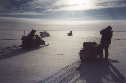
- Sea Ice extent
- Solar influence on climate
- The Little Ice Age and Medieval Warm Period
- Arctic Oscillation and sea ice
- Advanced statistical tools and methods
- Glaciology research
Geoengineering and Earth System Modelling
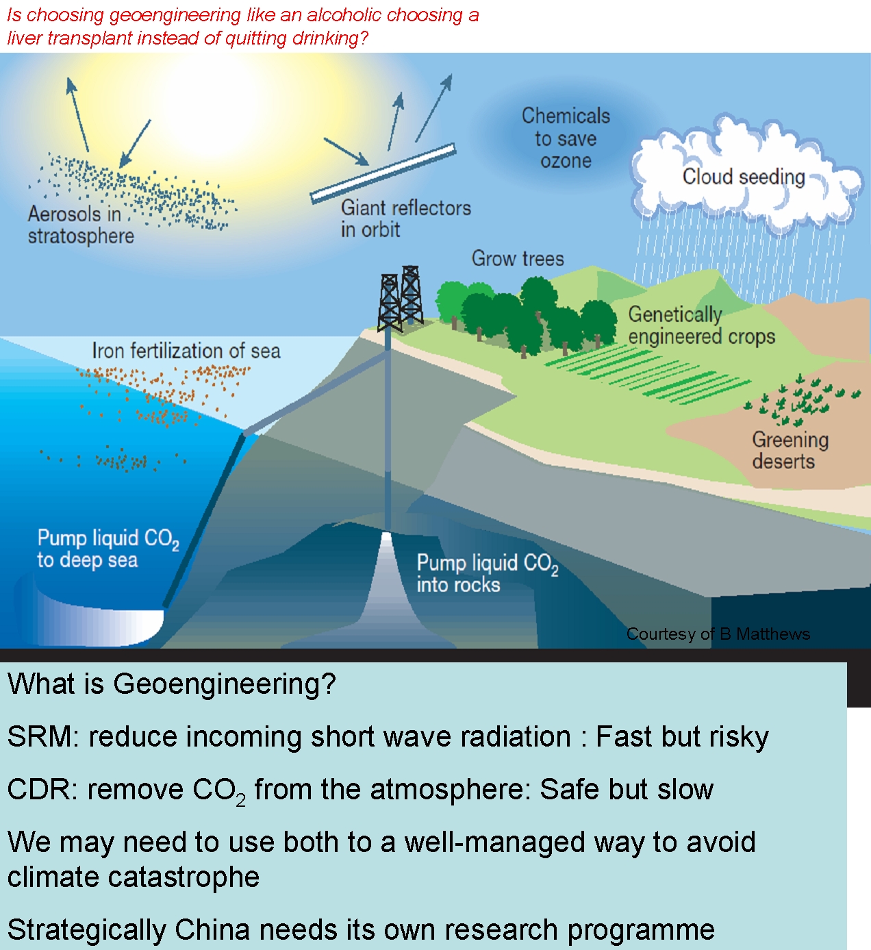
I lead China's research program in geoengineering. This is a key research program fuded under the Global Change Research Fund from the Ministry of Science and Technology (known as a "973 project".)We look at many aspects of geoengineering from the basic mechanisms, through Earth System Models and integrate it with socio-economic and governance aspects.
In particular we are interested in looking at combined methods of geoengineering - that is explore how spatial and seasonally varying methods may interact with eachother and the climate system.
We are also keen to focus on the impacts of geoengineering - such as on extreme events, agriculture, and society as it decarbonizes. We think that Chinese experience of megaengieering may also be useful in establishing governence paths for geoengineering.
An example of impact research comesfrom a new paper in PNAS on the impact of how geoengineering may impact Atlantic hurricanes.
We looked at the role of geoengineering in reducing possible 21st century sea level rise in a 2010 PNAS paper. This showed that indeed geoengineering could reduce sea level by perhaps 30 cm or so (depending on how agressively it was done). Of course a key element in geoengineeering are the unexpected side effects that can occur as the long wave absorbtion of energy by greenhouse gases is often balanced by reduction in incoming solar short wave radiation by e.g. stratospheric aerosol particle injection.
In fact much more difficult than even the challenging technological issues involved in geoengineering are the political issues of securing international agreement on such deliberate actions - where inevitably countries will be relative winner and loosers.
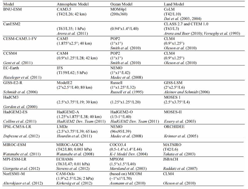
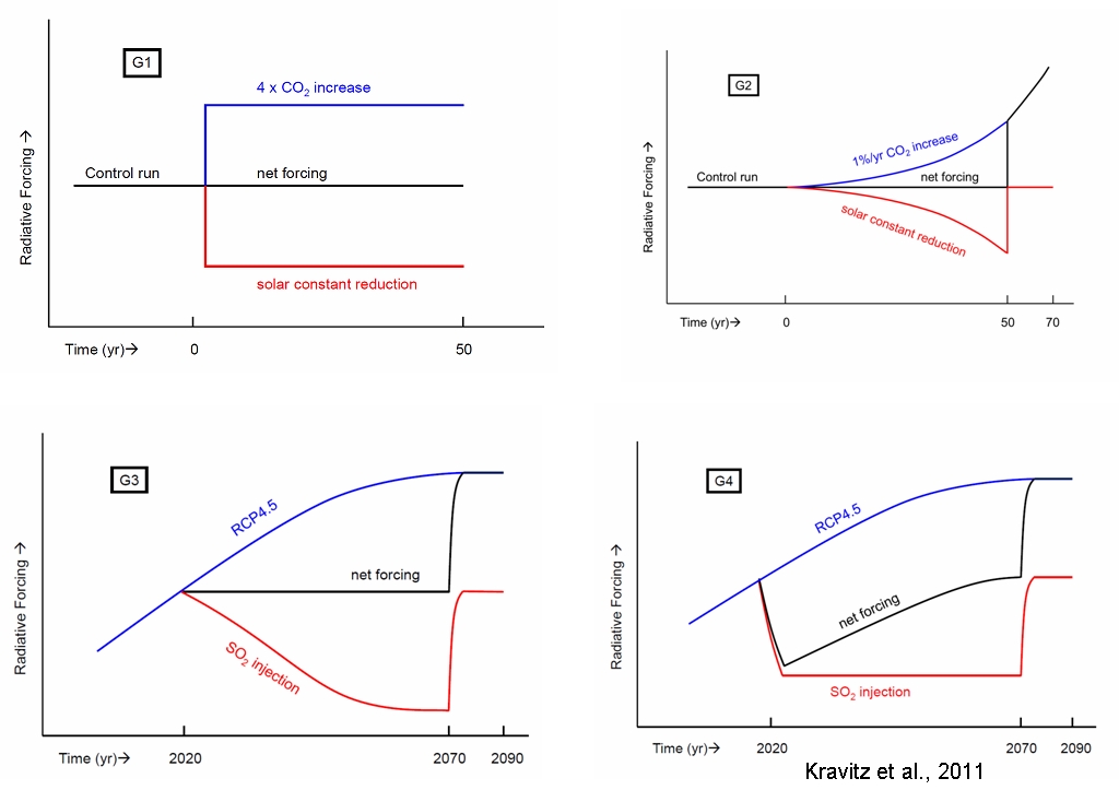
We can look at the various possibilities of geoengineering using earth System Models - and in Beijing we have developed on and used it for the new IPCC simulations (stored in the CMIP5 archive).
For geoengineering there is a similar set of scenarios called Geomip. And results from 12 models are being processed and interpretted now.
Geoengineering Research at GCESS:
Arctic sensitivities: sea ice, ice sheets, permafrost
China impacts: sea level rise, socioeconomic, international governance
Focus on: extreme events, ice-ocean interactions, deserts and albedo, oceans, permafrost model improvement
Funding from Cooperation Centre of Global Change at Beijing Normal University
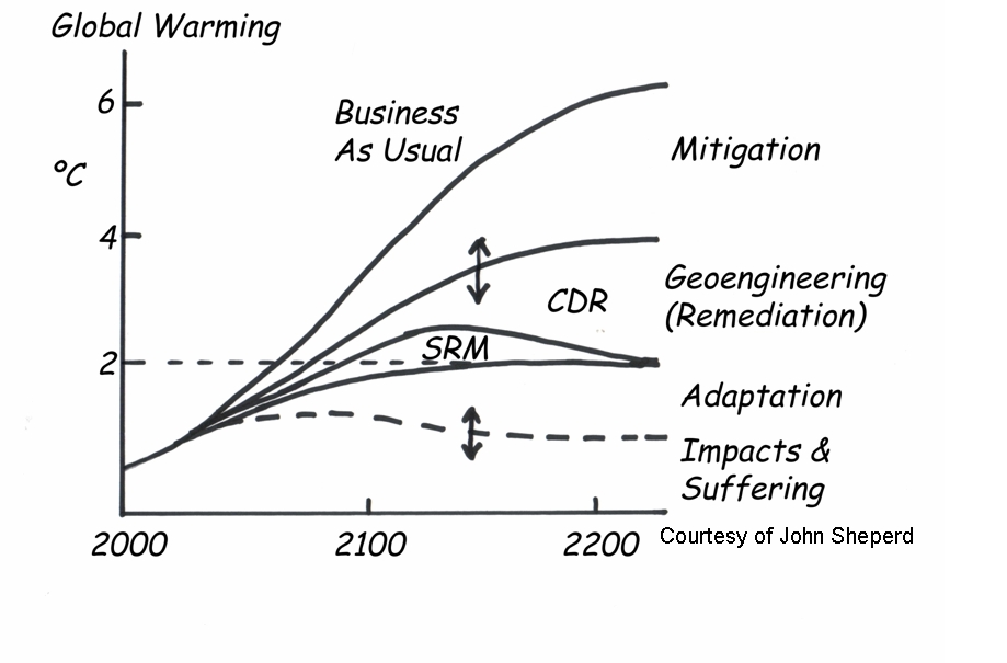
The moral responsibilities of different countries for past climate change, and their obligations to climate mitigation are also key here. Indeed if climate mitigation through reduction of greenhouse gases does not occur in the next decades then the world will either suffer the damaging consequences of dramatic climate change, or the impact of risky geoengineering.
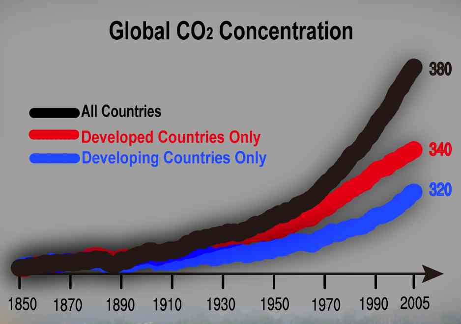
Using the earth system models from BNU and the CESM (developed by NCAR in Boulder) we explored how sea ice, ocean temperatures, snow cover and surface temperatures would have varied if CO2 had been emitted by only developed countries (defined in the IPCC Annex 1) and compared the impacts with those if CO2 had come from only the developing world (non Annex 1 countries). The results show that the developed world contributes about 2/3 to climate chnage while developing world about 1/3. This is despite the fact that most growth in emissions comes from developing world countries (like China). The reason is of course that the oceans and sea ice etc take some time to respond to the driving from the greenhouse gases. So the much earlier emissions form the developed world are important in the on-going climate change. We also looked at how the climate system would respond in future to the committments that countries signed on to at Cancun. This shows that developed world commitments would only reduce climate chnage by about half as much as the committments from the developing world. That is the developed world is signing on to cut climate change impacts by 1/3 and developing world 2/3. This is not an equitable division given their historical climate change responsibilities.
Hurricanes and extreme events
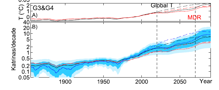
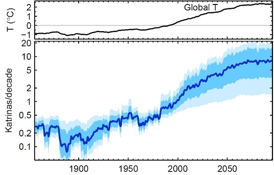
Linkages between hurricanes and climate warming are controversial. This is largely because most economic damage is not done by gradual change in mean climate such as sea level rise, even though the gradual accumulation of such change is almost certainly catastrophic - but by extreme events. Hurricanes, especially in the Atlantic are one area where climate science has enormous political impact. Naïve expectations from climate models are that hurricanes numbers would not increase very quickly with rising temperatures - however we much prefer using observational records than models to determine what is happening to the climate rather than what a computer program predicts.Two new papers in PNAS ("A new homogeneous record of Atlantic cyclone surge activity since 1923" and "Projected Atlantic tropical cyclone threat from rising temperatures") show unequivocally the link between warming and hurricane frequency. Using observations of Atlantic hurricanes during the past 80 years we found a strong relationship between the coastal flood surges these storms cause and surface temperatures. The relationship allow us to use Earth System models to see how the frequency of the will change in the future. We find that the largest storms are most sensitive to rising temperatures. The famous hurricane Katrina in 2005 caused great damage to New Orleans, and we find that storm surge floods of these magnitude become 10 times more likely if the average global temperature becomes 2C warmer.
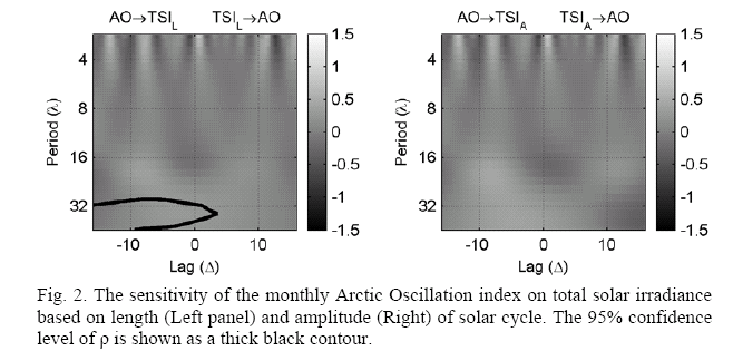
We have used the same kinds of advanced statistical methods we used to demonstrate the lack of a significant sunspot cycle link with Arctic Oscillation & ENSO, to examine large Atlantic tropical storms, ENSO, and warming tropical Atlantic temperatures. One paper is in Journal of Climate, another in a Springer volume. So what we can publish here is limited. However what we can say is that there is a causal relationship between warming Atlantic temperatures and frequency of large tropical Atlantic storms, that the ameliorating effects of ENSO on Atlantic storms has diminished in importance, and that export of warmth by the Atlantic drift current/North Atlantic Oscillation seems to decreased since the 1980s. This means that rising temperatures are causing more Atlantic storms (and most likely the extreme storms that become hurricanes).
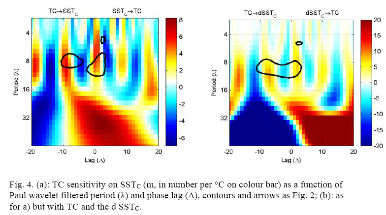
This graph shows that sea surface temperatures in the tropical Atlantic significantly decreasing numbers of tropical cyclones at 5 yearly (due to ENSO) but significantly rising cyclone numbers at decadal periods, (the red colours in the black contoured regions at positive lags in the left hand figure) Furthermore the right hand panel shows that there is feedback present whereby more tropical cyclones slow the rate of rising temperature.
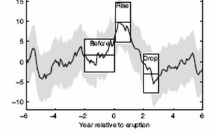
Another type of extreme event that we have studied are the large volcanic events - their impact on global sea level, and also the impact of the 1783 eruption of Laki in Iceland.
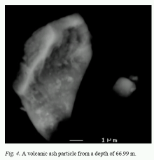 This was a very large fissure eruption - not an explosive event,
but a nearly year-long eruption that released a tremendous amount of acidic gasses
that killed much of the livestock on Iceland and perhaps 20 000 people in Europe
as the plume was carried down wind.
Our Lomonosovfonna ice core from Svalbard
contained tephra particles (the thick vertical line) from the eruption, and a large sulphuric acid peak (thick line).
This was a very large fissure eruption - not an explosive event,
but a nearly year-long eruption that released a tremendous amount of acidic gasses
that killed much of the livestock on Iceland and perhaps 20 000 people in Europe
as the plume was carried down wind.
Our Lomonosovfonna ice core from Svalbard
contained tephra particles (the thick vertical line) from the eruption, and a large sulphuric acid peak (thick line).
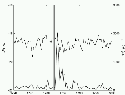 Interestingly the eruption cooled the climate for several years at least in the
Barents region (thin grey line), and there are reports of anomalous conditions in the Atlantic
for a decade after the eruption. Certainly analysis of the sulphate in the ice
core record indicates that decades after the eruption were the only period of
the Little Ice Age to appear as atmospherically acidic as the 20th Century.
Interestingly the eruption cooled the climate for several years at least in the
Barents region (thin grey line), and there are reports of anomalous conditions in the Atlantic
for a decade after the eruption. Certainly analysis of the sulphate in the ice
core record indicates that decades after the eruption were the only period of
the Little Ice Age to appear as atmospherically acidic as the 20th Century.
Sea level
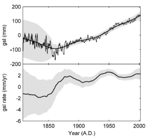
Moore et al 2011 examine the sea level budget since 1850. This is interesting becuase there has been a problem in assigning the observed rates of sea level rise from tide gauges or sattelites with the best estimates from the different components such as ice sheet and glacier melt, thermal expansion of sea water, terrestrial inflow from groundwater extraction etc. Good estimates of sea-level contributions from glaciers and small ice caps, the Greenland ice sheet and thermosteric sea level are available over this period, though considerable scope for controversy remains in all. Attempting to close the sea-level budget by adding the components results in a residual displaying a likely significant trend of .0.37mma¨C1 from 1955 to 2005, which can, however, be reasonably closed using estimated melting from unsurveyed high-latitude small glaciers and ice caps. The sea-level budget from 1850 is estimated using modeled thermosteric sea level and inferences from a small number of mountain glaciers. This longer-term budget has a residual component that displays a rising trend likely associated with the end of the Little Ice Age, with much decadal-scale variability that is probably associated with variability in the global water cycle, ENSO and long-term volcanic impacts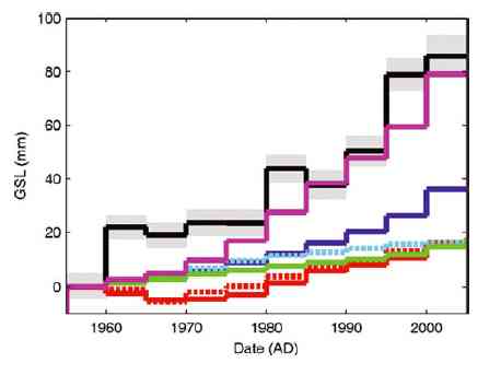
Time series of anomalies in sea-level components from 1955 to 2005. GSL (black, with standard error as grey shaded region (Jevrejeva et al, 2006)); TS (red solid line, from Domingues et al (2008) corrected for full ocean depth); modeled thermosteric (red dotted line (Gregory et al, 2006)). Cumulative mass balance as sea-level equivalents for: GSIC (blue; Cogley, 2009), GIS (green; Rignot et al. 2008a) and mountain glacier termini (cyan; Oerlemans et al., 2007). Also shown are summed components (TS + GSIC + GIS + PSG; magenta). The 1955¨C60 period is the baseline for all datasets
We made what we think is the best global sea level reconstruction. We think it's the best because
- 1. it uses all the tide station data available in the most sensible and optimal way
- that is it uses a method we call the "virtual station" approach - this
compensates for the fact that many stations exist around Europe and North America,
while few stations and relatively recently measured sea level in the Southern Hemisphere.
- 2. We compute the global curve from sets of regional curves that cover 13 separate
oceanic regions - this allows changes in e.g. the Gulf Stream which can mean that
the western and eastern North Atlantic have quite different sea level behavior
over time can be averaged together sensibly.
- 3. The resulting curve captures some very interesting effects such as what large
 tropical volcanic eruptions do to the water cycle. Previous sea level reconstructions
do not show any significant features due to large volcanic effects - although
simple models predict that sea level should fall after an eruption.
In fact our sea level curve shows that sea level rises for about 1 year
and then falls for several years after that. For a simple explanation of the mechanism
read our press release, and for more details
read the whole article and its supplementary material.
tropical volcanic eruptions do to the water cycle. Previous sea level reconstructions
do not show any significant features due to large volcanic effects - although
simple models predict that sea level should fall after an eruption.
In fact our sea level curve shows that sea level rises for about 1 year
and then falls for several years after that. For a simple explanation of the mechanism
read our press release, and for more details
read the whole article and its supplementary material.So for these reasons we think our data is the best to use for anyone wanting to explore sea level history over the last 200 years.
21st century Sea level
Sea level will rise more than expected
Our paper in Climate Dynamics, shows our projections for 2100 based on inverse modelling sea level from tide gauges to temperature reconstructions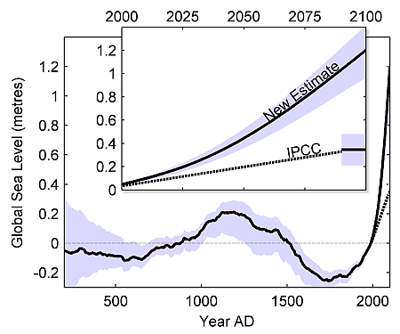 and historical temperature data over the past two millennia. The article is here,
and the press release with some nice images is here
Sea level rise is one of the most important impacts of a changing climate.
Municipalities in Finland have announced plans to strengthen their sea defences,
but it is worthwhile highlighting recent scientific analysis of sea level.
Sea level will rise due to rising temperatures via: expansion of water as its
temperature rises, and increasing mass of water in the oceans as ice sheets and
glaciers melt. The IPCC scientific assessment - which was based on scientific
articles published before mid 2006, meaning science done in 2005 -
estimated that about 2/3 of present increase was due to thermal expansion of
ocean water. IPCC estimated that 2100 sea level would rise between about 20-60 cm
(depending on how fast temperatures increase). However, since the IPCC report was issued,
measurements from satellite altimetry show that sea level rise is accelerating
so that the rise rate over the last 3 years is 4 mm/year, while the 20th Century
average was 1.8 mm/year. Furthermore, almost all of the increase appears to be
due to mass loss from the large Greenland and Antarctic ice sheets. This means
that actually thermal expansion amounts for only 1/3 of sea level rise,
melting of ice is dominating sea level rise and will become increasing important.
and historical temperature data over the past two millennia. The article is here,
and the press release with some nice images is here
Sea level rise is one of the most important impacts of a changing climate.
Municipalities in Finland have announced plans to strengthen their sea defences,
but it is worthwhile highlighting recent scientific analysis of sea level.
Sea level will rise due to rising temperatures via: expansion of water as its
temperature rises, and increasing mass of water in the oceans as ice sheets and
glaciers melt. The IPCC scientific assessment - which was based on scientific
articles published before mid 2006, meaning science done in 2005 -
estimated that about 2/3 of present increase was due to thermal expansion of
ocean water. IPCC estimated that 2100 sea level would rise between about 20-60 cm
(depending on how fast temperatures increase). However, since the IPCC report was issued,
measurements from satellite altimetry show that sea level rise is accelerating
so that the rise rate over the last 3 years is 4 mm/year, while the 20th Century
average was 1.8 mm/year. Furthermore, almost all of the increase appears to be
due to mass loss from the large Greenland and Antarctic ice sheets. This means
that actually thermal expansion amounts for only 1/3 of sea level rise,
melting of ice is dominating sea level rise and will become increasing important.
Sea level 200-2100 AD
Extrapolating sea level using IPCC projections of temperature rise due to greenhouse emission to 2100 (a rise of about 2C) leads us to estimate sea level about 1-2 m higher than at present, with essentially nil probability of rises as low as 60 cm. This rate of sea level rise is quite consistent with what we know of how fast sea level rose as the large ice sheets melted at the end of the last ice age. Between 14000 and 7000 years ago sea level rose by 1.1 m/century on average. Additionally, sea level rose by 10 m within centuries on at one occasion. Recent acceleration of ice flow and larger areas of melting over Greenland may indicate on-going and unexpectedly rapid decay of the ice sheet, through it may be decay is limited to the margins of ice sheet releasing less than the 7 m of global sea level rise that would occur if the whole ice sheet melted. Perhaps an even greater concern than Greenland is the 10 m of sea level equivalent locked away in the West Antarctic ice sheet. This ice sheet is grounded below sea level, and potentially liable to runaway collapse with rising sea levels.
Our sea level reconstruction since 200AD shows some remarkable findings- A Relatively consistent picture of LIA/MWP sea level despite very different temperature reconstructions
- Sea level is at present slightly lower than during the MWP
- Sea level 2100 will by far exceed anything seen the last 2000 years.
- IPCC much too conservative (although they do acknowledge that)
- Effective response time of sea level at present is a few centuries only
- A dynamic response from ice sheets likely began in the 1950s and is part of the underestimate of sea level rise components
This means that no matter what we do to reduce CO2 then we are already committed to a considerable rise in sea level. There is simply so much inertia in the system, because the ice masses and ocean heat have not equilibrated to surface temperatures. We must therefore adapt (by good infrastructure planning) to higher sea level. It sounds very controversial to project such a large rise but it really is not. see also this list of papers.
Causes of sea level rise
Jevrejeva,et al 2012 make projections of future sea level to the year 2500 using our semi-empirical model based on radiative forcing and using the new IPCC AR5 RCP scenarios that replace the earlier SRES ones.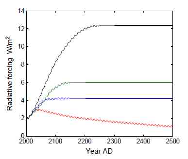
The figure shows Radiative forcings for the RCP scenarios; red¡ª RCP3PD, blue¡ª RCP4.5, green¡ª RCP6 and black ¡ª RCP8.5 from present day to AD2500. Note that the RCP8.5 is essentially a business as usual projection of economic growth, while the RCP3PD scenario implies use of geoengineering to reduce radiative forcing by mid 21st century. These scenarios are more "optimistic" than those used in the 2007 IPCC AR4 report.
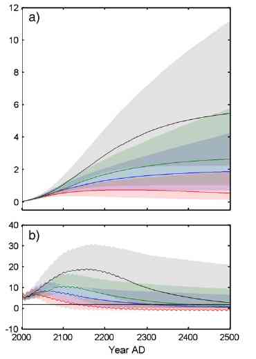
The next figure shows (a) Sea level projections by 2500 (in metres of global sea level) with RCP scenarios; red¡ª RCP3PD, blue¡ª RCP4.5, green¡ª RCP6 and black ¡ª RCP8.5. Shadows with similar colour around projections are upper (95%) and low (5%) confidence level. (b) Rates of sea level rise in mm/yr (colour scheme the same as panel a). The black horizontal line corresponds to the rate of sea level rise during the 20th century (1.8 mm/yr).
Note that the sea level for most scenarios continues to rise well beyond 2100, that projections have large uncertainties, that the rate of sea level rise likely peaks after 2100 and that it takes several hundred years for rates of rise fall back to those of the 20th century. These results have profound implications for infrastructure planning.
Jevrejeva et al 2009 developed a semi-empirical model for sea level as a function of radiative forcing. This shows that human activities have dominated global sea level since 1850.
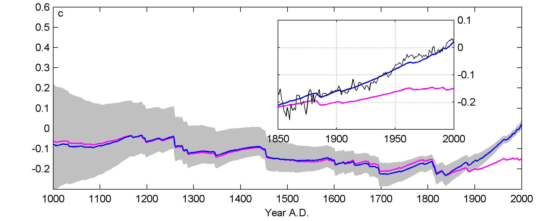 The causes of sea level variability are essentially driven by changes in global temperature, with a century-scale time delay because it takes time for the oceans to warm and ice to melt or glaciers grow. The changes in temperature are driven by both natural variability - changes in solar radiation reaching the Earth and volcanic eruptions, which cool the Earth by blocking incoming sunlight; and man-made causes such as greenhouse gases (warming the planet) and aerosols from pollution, which cause cooling.
There has been some controversy in deciding the relative amount of natural variability in the Earth's temperature compared with the man-made forcing. So instead of estimating global temperature, we looked directly at global sea level and the individual driving force components over the last 1000 years.
We find that until 1800 the main drivers of sea level change are volcanic and solar forcings.
The blue curve shows the sea level history for the last 1000 years when driven by both natural and man-made forcing factors, the pink curve shows the sea level resulting from only natural forcing. The inset shows the more recent period with the black curve being the observed global sea level variability measured by tide gauge stations
However, for the past 200 years sea level rise is mostly associated with anthropogenic factors. Only 4 cm (25% of total sea level rise) during the 20th century is attributed to natural forcings, the remaining 14 cm are due to a rapid increase in CO2 and other greenhouse gases. This is much larger than the impact of the volcanic eruptions which have produced a net lowering of about 7cm compared with levels expected if there had been no eruptions in the 20th century. It is possible that the man was already affecting sea level well before the large emissions of industrial greenhouse house gases by the change in land use and farming practices around the world.
Storm surges
Mean sea level is only one aspect of climate change that affects coastal infrastructure. Most damage is done by extreme events like hurricanes, storm surges and floods. A naïve expectation is that simply changing the mean temperature shifts the frequency of extreme events by a corresponding amount. However, a changing climate means that the frequency of extremes is not simply related to those we experienced in a different climate. Atlantic tropical cyclones (large storms that include hurricanes), tend to increase in frequency in warming climates. Furthermore since warmer climates have more energy, the largest events are more energetic - in the same way that a pan of water roils and moves more vigorously as its approaches boiling. Hence recurrence times for large floods may in a future climate be much shorter. The floods must be added to the increases in mean sea level, perhaps 1.5 m higher than now by the end of this century. The rules at present in Finland reflect IPCC assessments of sea level rise, and limit infrastructure less than 2.4 m above present sea level. Is this sufficiently precautionary a level considering that some planned installations need to survive well beyond the end of the century?
Sea Ice extent
A new paper in Climate Dynamics by Macias et al discusses sea ice in the region east of Greenland over the last 800 years. The minimum annual extent of Arctic sea ice has dropped significantly since about 1980. The maximum annual extent has received less coverage than the annual minimum; this plot shows the satellite time series to 2008 from 2 different instruments.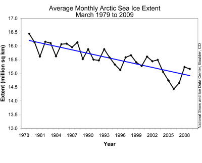 Of course the direct observation period is limited. Indirect observations come
from ships that recorded the ice edge location in their logs and which extends,
in the European Arctic, back to 1864 (Vinje, 2001), and sporadically back to about 1600.
Naturally its interesting to extend that record, especially in the light of the
natural variability expected from The Little Ice Age and Medieval Warm Period.
Of course the direct observation period is limited. Indirect observations come
from ships that recorded the ice edge location in their logs and which extends,
in the European Arctic, back to 1864 (Vinje, 2001), and sporadically back to about 1600.
Naturally its interesting to extend that record, especially in the light of the
natural variability expected from The Little Ice Age and Medieval Warm Period.
We constructed a proxy for sea ice extent from the supra-long (7500 year) Scandinavian tree ring chronology (Eronen et al., 2002) and the Lomonosovfonna oxygen isotope record (Isaksson et al. 2005). Interestingly when we did this we found the best fit was not with the minimum ice extent that occurs around September, but with the annual maximum which occurs around April, and in the area west of 10E - the western Nordic Seas - that is the region east of Greenland. At first glance predicting maximum ice which depends on winter severity seems puzzling since trees only grow in summer. Relationships between winter climatic conditions and tree growth in northern Fennoscandia have been previously reported (e.g. DArrigo et al. 1993): winter sea-ice extent and sea-level pressure can persist into the spring and summer months, when climate is exerting a more direct influence on tree growth (Cook et al. 1998). Ice core records form Svalbard seem to preserve a reasonable record containing information on the whole year's snow fall (Pohjola et al., 2002) - though seasonal melting each summer blurs the time resolution available to a few years (Moore et al., 2005).
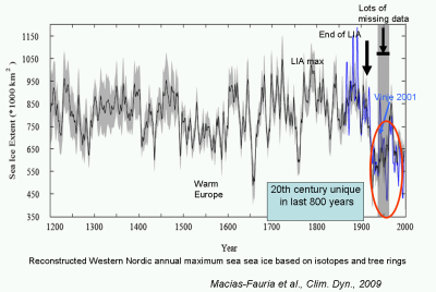 Our reconstruction using a callibration-verification method - splitting the target time series (the obsevered sea ice extent from Vinje, 2001)
explains about 59% of the variance, and is skillful. in other words it has statistical value outside the callibration period.
The figure shows by a blue line historical maximum sea ice
extent in the Western Nordic Seas (Norway, Iceland and Greenland
Seas; Vinje 2001) during 18641997. The period 19401959,
obtained mainly from interpolation due to abundant missing data
is highlighted by a grey shaded rectangle;
black line: multiproxy reconstruction of sea ice extent in the Western
Nordic Seas during 12001997; grey shaded area: area within the
95% confidence interval of the reconstruction.
Our reconstruction using a callibration-verification method - splitting the target time series (the obsevered sea ice extent from Vinje, 2001)
explains about 59% of the variance, and is skillful. in other words it has statistical value outside the callibration period.
The figure shows by a blue line historical maximum sea ice
extent in the Western Nordic Seas (Norway, Iceland and Greenland
Seas; Vinje 2001) during 18641997. The period 19401959,
obtained mainly from interpolation due to abundant missing data
is highlighted by a grey shaded rectangle;
black line: multiproxy reconstruction of sea ice extent in the Western
Nordic Seas during 12001997; grey shaded area: area within the
95% confidence interval of the reconstruction.
The results of the analysis allow us to look at maximum annual sea ice extent in the Western Nordic seas over about 800 years
Notable findings are:
- 1 The 20th century lowest maximum sea ice extent values since A.D. 1200.
- 2 The presently low maximum sea ice extent in the Western Nordic Seas is
unique over the last 800 years, and results from a sea ice decline started in mid-19th century after the Little Ice Age.
Solar influence on climate
Recently there have been many papers on solar forcing. Many climate skeptics view solar forcing as the main driver of climate change on decadal time scales. IPCC does not share that view, and the results from my research supports IPCC.Many groups use simple correlations to try to show that the 11 year sun spot cycle affects all kinds of climate (and many other) variables on earth. In contrast we use causality rather than simple correlation methods. By causality I mean that one variable can be said to cause another variable if at all times the prediction using a different time series is better than obtained using previous values of just one time series.
Causality testing that if half the time one series peaks slightly before another while at other times it peaks slightly later,then the two series would not be causal (in the Granger sense), whereas they could well be significantly correlated. I have written two articles #91 and #83, that do not support any significant signal from solar forcing on large scale climate patterns (the Arctic Oscillation or ENSO) that are main actors in global climate.
Interestingly the same methods do show a causal link between ENSO and Arctic Oscillation. That is discussed in the Arctic Oscillation and sea ice section.
The Little Ice Age and Medieval Warm Period
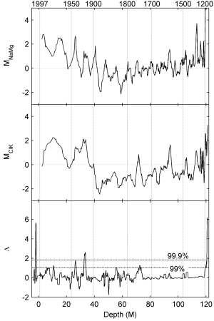
Another controversial climate issue concerns how similar is the present day climate to warm episodes in the past: in other words is what we are seeing today simply a natural climate oscillation. In many ways of course the answer is not very helpful since a thousand or more years ago there was very little infrastructure that was likely to be affected by climate change compared with today. However the question is certainly interesting scientifically.We have studied via the Lomonosovfonna ice core, the climate and environment around Svalbard over the last 800 years. I have co-authored at least 20 papers on this ice core record - and my group has mainly dealt with the chemical analysis of the core, and the mathematical analyses such as the dating of the core and the extraction of subtle features in the various time series.
We had a lot of obstacles to overcome in getting the record accepted by the scientific community as the ice core suffers from seasonal melting whereby some of the snow is converted to ice each summer. We showed that this tends to smooth signals with time, though only by a few years, so in reality this ice core is just as reliable for most records as ones from central Greenland or Antarctica.
Some of our findings have been surprising - we find that most of the anthropogenic (industrial) sulphur deposited on the ice cap comes from western Europe, and not the large industrial regions of Norilsk or the Kola Peninsula. This is most likely because of the strong inversion that exists close to sea level that prevents Arctic Haze pollution from reaching the core site, so in some ways the drill site appears to be located much higher in the atmosphere than the 1200 m actual height.
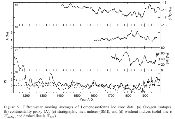 Other analyses
show that the Little Ice Age winter and spring season climates
changed at different rates. Most likely reflecting changes in sea ice extent.
The continentality decreased before the temperatures started to rise, indicating
that sea ice retreated making the island more maritime 20-30 years before yearly
temperatures started to rise. Summer melting was also
modelled
based on the relative
elution of pairs of ions - some ions are removed from ice to liquid easier than
others - and we found that melting was greater 1130-1300 than in the 20th Century.
Other analyses
show that the Little Ice Age winter and spring season climates
changed at different rates. Most likely reflecting changes in sea ice extent.
The continentality decreased before the temperatures started to rise, indicating
that sea ice retreated making the island more maritime 20-30 years before yearly
temperatures started to rise. Summer melting was also
modelled
based on the relative
elution of pairs of ions - some ions are removed from ice to liquid easier than
others - and we found that melting was greater 1130-1300 than in the 20th Century.
 However we returned to Lomonosovfonna in the years following the ice coring,
and two new papers (1) (2) compare what we observe in the snow pits that sample the firn
layers deposited in the 21st Century. Now we find that the recent years are very
comparable to the early years of the core, and that conditions are now close to
summer conditions in the Medieval warm Period on Svalbard.
However we returned to Lomonosovfonna in the years following the ice coring,
and two new papers (1) (2) compare what we observe in the snow pits that sample the firn
layers deposited in the 21st Century. Now we find that the recent years are very
comparable to the early years of the core, and that conditions are now close to
summer conditions in the Medieval warm Period on Svalbard.This is relevant to discussions of how sensitive and how quickly glaciers melt in warmer conditions, and what global sea level may have been over the last thousand year. We believe that we have good estimates of that, and that sea level was not much different than today. However during the rest of the 21st Century temperatures are expected to rise rapidly by at least 2C globally - and most likely by much more in the Arctic and Antarctic regions.
Arctic Oscillation and sea ice
One way of looking at global climate is actually made up of large patterns such as ENSO which represent the thermal state of the upper tropical Pacific Ocean, or the Annular Modes such as the Arctic (AO) Oscillation that are essentially determined by the strength of the polar stratospheric vortices. These large scale patterns of variability represent the largest climate mechanisms on the planet. Therefore analyzing their behaviour leads to an understanding of how climate operates, and can also provide clues on what a different climate may work like given the observed sates of these mechanisms during the past.Our work on the large circulation patterns was prompted by studies of sea ice - initially in the Baltic Sea where records extend back in time to the 1700s due to the economic importance of the ice season. Later we extended the analysis to the Barents Sea, and also looked at many other variables such as sea surface temperatures and pressures, and sea level records.
Europe has traditionally been seen as a region where ENSO has little measurable impact, but the impact of the characteristic biannual and multi-year ENSO oscillations can be seen in the Baltic Sea ice record (BMI). Perhaps most striking is the 14-year oscillation which is shown varying in importance over time.
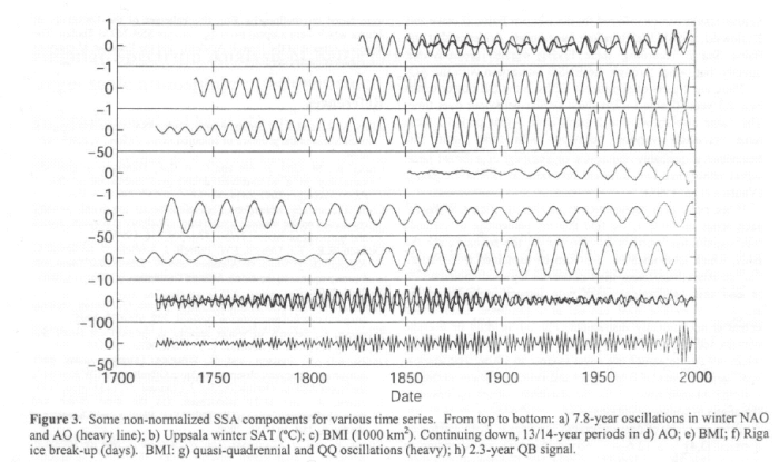
We traced this 14 year signal in sea surface temperatures from its origin in
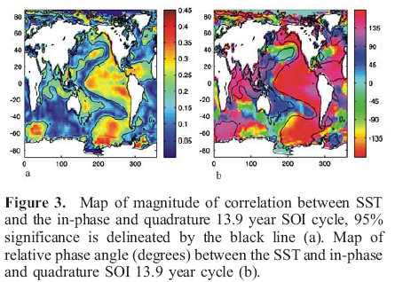 the central Pacific as it moves eastwards and then along the coast of the Americas
to the polar regions. It takes about 2 years for the signals to travel around
the planet, and show a slow linkage between tropics and polar regions.
the central Pacific as it moves eastwards and then along the coast of the Americas
to the polar regions. It takes about 2 years for the signals to travel around
the planet, and show a slow linkage between tropics and polar regions.In contrast the tropical signals with 2-5 year periods arrive in the polar regions faster. After only 2-3 months, indicating a fast transport path through the atmosphere.
These long period signals propagating around the planet mean that some data sets such as sea level records can be very sensitive to changes in these patterns - particularly the changes caused by Arctic Oscillation. We find that for some places such as Northern Europe, that up to 35% of the sea level record is caused by changes in these large circulation patterns, which drive ocean currents and the tracks of depressions across the Atlantic. These same patterns cause Atlantic water to be driven into the Arctic Ocean, resulting in large changes in ecosystems in the Arctic, and of course contributing the decline in Arctic sea ice.